Genome annotation
The Rfam library of covariance models can be used to search sequences (including whole genomes) for homologues to known non-coding RNAs, in conjunction with the Infernal software.
Before trying to annotate your own genome sequences on your local hardware or submitting lots of sequences to Rfam via the website, please check that the following resources do not provide the annotation for you:
Hint
For more details about genome annotation, please see our paper in Current Protocols in Bioinformatics or follow a Docker-based tutorial showing how to annotate a viral genome with RNA families.
Example of using Infernal and Rfam to annotate RNAs in an archaeal genome
The instructions below will walk you through how to annotate the Methanobrevibacter ruminantium genome (NC_013790.1) for non-coding RNAs using Rfam and Infernal. The files needed are included in the Infernal software package, which you will download in step 1.
Download, build and install Infernal from http://eddylab.org/infernal/
wget eddylab.org/infernal/infernal-1.1.2.tar.gz
tar xf infernal-1.1.2.tar.gz
cd infernal-1.1.2
make
If you do not have wget installed and in your path, download infernal-1.1.2.tar.gz here.
To compile and run a test suite to make sure all is well, you can optionally do:
make check
You don’t have to install Infernal programs to run them. The newly compiled binaries are now in the src directory. You can run them from there. To install the programs and man pages somewhere on your system, do:
make install
By default, programs are installed in /usr/local/bin and man pages
in /usr/local/share/man/man1/. You can change the /usr/localprefix to
any directory you want using the ./configure
--prefix option, as in ./configure --prefix /the/directory/you/want.
Additional programs from the Easel library are available in easel/miniapps/. You can install these too if you’d like. Step 4 below involves the use of one of these Easel programs (esl-seqstat). If you do not install these programs, you can use the executable files in easel/miniapps/. To install them:
cd easel; make install
For more information on customizing the Infernal installation, see section 2 of the Infernal User’s Guide.
Download the Rfam library of CMs from https://ftp.ebi.ac.uk/pub/databases/Rfam/CURRENT/Rfam.cm.gz and the Rfam clanin file from https://ftp.ebi.ac.uk/pub/databases/Rfam/CURRENT/Rfam.clanin .
wget ftp://ftp.ebi.ac.uk/pub/databases/Rfam/CURRENT/Rfam.cm.gz
gunzip Rfam.cm.gz
wget ftp://ftp.ebi.ac.uk/pub/databases/Rfam/CURRENT/Rfam.clanin
If you do not have wget installed and in your path, download the
files https://ftp.ebi.ac.uk/pub/databases/Rfam/CURRENT/Rfam.cm.gz and
https://ftp.ebi.ac.uk/pub/databases/Rfam/CURRENT/Rfam.clanin
from a browser.
Use the Infernal program cmpress to index the Rfam.cm file
cmpress Rfam.cm
This step is required before cmscan can be run in step 5.
Determine the total database size for the genome you are annotating.
For the purposes of Infernal, the total database size is the number of nucleotides that will be searched, in units of megabases (Mb, millions of nucleotides). So, it is the total number of nucleotides in all sequences that make up the genome, multiplied by two (because both strands will be searched), and divided by 1,000,000 (to convert to millions of nucleotides).
You will need to supply this number to Infernal to assure that the E-values reported by the cmscan program run in the next step are accurate.
You can use the esl-seqstat program from the Easel library that you built along with Infernal in step 1 to help with this. For this example, we will be annotating the genome of Methanobrevibacter ruminantium, an archaeon. The sequence file with this genome can be found in infernal-1.1.2/tutorial/, which you created in step 1. To determine the total size of this genome, do:
esl-seqstat infernal-1.1.2/mrum-genome.fa
Note
If you did not install the Easel miniapps in step 1, you can
run esl-seqstat from infernal-1.1.2/easel/miniapps/esl-seqstat.
The output will include a line reporting the total number of nucleotides:
Total # of residues: 2937203
Because we want millions of nucleotides on both strands, we multiple this by 2, and divide by 1,000,000 to get 5.874406. This number will be used in step 5.
Use the cmscan program to annotate RNAs represented in Rfam in the Methanobrevibacter ruminantium genome.
cmscan -Z 5.874406 --cut_ga --rfam --nohmmonly --tblout mrum-genome.tblout --fmt 2 --clanin Rfam.clanin Rfam.cm tutorial/mrum-genome.fa > mrum-genome.cmscan
Note
The above cmscan command assumes you are in the infernal-1.1.2 directory from step 1. If not, you’ll need to supply the paths to the tutorial/mrum-genome.fa and file within the infernal-1.1.2 directory.
Explanations of the command line options used in the above command are as follows:
-Z 5.874406the sequence database size in millions of nucleotides is 5.874406, it is the number computed in step 4. This option ensures that the reported E-values are accurate.
--cut_gaspecifies that the special Rfam GA (gathering) thresholds be used to determine which hits are reported. See more in the section Gathering cutoff.
--rfamrun in “fast” mode, the same mode used for Rfam annotation and determination of GA thresholds
--nohmmonlyall models, even those with zero basepairs, are run in CM mode (not HMM mode). This ensures all GA cutoffs, which were determined in CM mode for each model, are valid.
--tblouta tabular output file will be created.
--fmt 2the tabular output file will be in format 2, which includes annotation of overlapping hits.
--claninClan information should be read from the file
Rfam.clanin. This file lists which models belong to the same clan. Rfam clans are groups of models that are homologous and therefore it is expected that some hits to these models will overlap. For example, the LSU rRNA archaea and LSU rRNA bacteria models are both in the same clan.
Remove hits from the tabular output file that have overlapping hits with better scores. This step is explained below after a discussion of the cmscan output, in the section: Removing lower-scoring overlaps from a tblout file.
Understanding Infernal output
The above cmscan command will take at least several minutes and
possibly up to about 30 minutes depending on the number of cores and
speed of your computer. After it has finished, you will have two
output files: mrum-genome.cmscan (standard output of cmscan) and
mrum-genome.tblout (tabular output).
cmscan standard output
The first section of Infernal program’s standard output is the header, telling you what program you ran, on what, and with what options:
 1# cmscan :: search sequence(s) against a CM database
 2# INFERNAL 1.1.2 (July 2016)
 3# Copyright (C) 2016 Howard Hughes Medical Institute.
 4# Freely distributed under a BSD open source license.
 5# - - - - - - - - - - - - - - - - - - - - - - - - - - - - - - - - - - - -
 6# query sequence file:                   /Users/nawrockie/src/infernal-1.1.2/tutorial/mrum-genome.fa
 7# target CM database:                    Rfam.cm
 8# database size is set to:               5.9 Mb
 9# tabular output of hits:                mrum-genome.tblout
10# tabular output format:                 2
11# model-specific thresholding:           GA cutoffs
12# Rfam pipeline mode:                    on [strict filtering]
13# clan information read from file:       Rfam12.2.claninfo
14# HMM-only mode for 0 basepair models:   no
15# number of worker threads:              8
16# - - - - - - - - - - - - - - - - - - - - - - - - - - - - - - - - - - - -
The second section is a list of ranked top hits (sorted by E-value,
most significant hit first). For cmscan output this section is
broken down per-query sequence. In this example, there is only one
sequence NC_013790.1. Here is the list of the top 25 hits (out of 78
total):
 1Query:       NC_013790.1  [L=2937203]
 2Description: Methanobrevibacter ruminantium M1 chromosome, complete genome
 3Hit scores:
 4 rank     E-value  score  bias  modelname                start     end   mdl trunc   gc  description
 5 ----   --------- ------ -----  ---------------------- ------- -------   --- ----- ----  -----------
 6  (1) !         0 2763.5  45.1  LSU_rRNA_archaea        762872  765862 +  cm    no 0.49  -
 7  (2) !         0 2755.0  46.1  LSU_rRNA_archaea       2041329 2038338 -  cm    no 0.48  -
 8  (3) !         0 1872.9  45.1  LSU_rRNA_bacteria       762874  765862 +  cm    no 0.49  -
 9  (4) !         0 1865.5  46.2  LSU_rRNA_bacteria      2041327 2038338 -  cm    no 0.48  -
10  (5) !         0 1581.3  41.5  LSU_rRNA_eukarya        763018  765851 +  cm    no 0.49  -
11  (6) !         0 1572.1  42.3  LSU_rRNA_eukarya       2041183 2038349 -  cm    no 0.49  -
12  (7) !         0 1552.0   4.1  SSU_rRNA_archaea       2043361 2041888 -  cm    no 0.53  -
13  (8) !         0 1546.5   4.1  SSU_rRNA_archaea        760878  762351 +  cm    no 0.54  -
14  (9) !         0 1161.9   3.7  SSU_rRNA_bacteria      2043366 2041886 -  cm    no 0.53  -
15 (10) !         0 1156.4   3.7  SSU_rRNA_bacteria       760873  762353 +  cm    no 0.53  -
16 (11) !  9.9e-293  970.4   4.6  SSU_rRNA_eukarya       2043361 2041891 -  cm    no 0.53  -
17 (12) !  9.9e-291  963.8   4.5  SSU_rRNA_eukarya        760878  762348 +  cm    no 0.54  -
18 (13) !  7.7e-281  919.9   4.6  SSU_rRNA_microsporidia 2043361 2041891 -  cm    no 0.53  -
19 (14) !  5.4e-280  917.2   4.5  SSU_rRNA_microsporidia  760878  762348 +  cm    no 0.54  -
20 (15) !   1.1e-53  184.9   0.0  RNaseP_arch            2614544 2614262 -  cm    no 0.43  -
21 (16) !   6.9e-49  197.6   0.1  Archaea_SRP            1064321 1064634 +  cm    no 0.44  -
22 (17) !   6.8e-28  115.2   0.0  FMN                     193975  193837 -  cm    no 0.42  -
23 (18) !   4.9e-16   72.1   0.0  tRNA                    735136  735208 +  cm    no 0.59  -
24 (19) !     1e-15   71.0   0.0  tRNA                   2350593 2350520 -  cm    no 0.66  -
25 (20) !   1.1e-15   70.9   0.0  tRNA                   2680310 2680384 +  cm    no 0.52  -
26 (21) !   2.2e-15   69.7   0.0  tRNA                   2351254 2351181 -  cm    no 0.62  -
27 (22) !   2.5e-15   69.5   0.0  tRNA                    361676  361604 -  cm    no 0.51  -
28 (23) !   3.2e-15   69.2   0.0  tRNA                   2585265 2585193 -  cm    no 0.60  -
29 (24) !   3.9e-15   68.8   0.0  tRNA                   2585187 2585114 -  cm    no 0.59  -
30 (25) !   4.3e-15   68.7   0.0  tRNA                   2680159 2680233 +  cm    no 0.67  -
The most important columns here are those labelled “E-value”, “score”, “modelname”, “start” and “end”, which are described below. For information on the other columns see the tutorial section (pages 18-19) of the Infernal User’s Guide).
E-valueThe E-value is the statistical significance of the hit: the number of hits we’d expect to score this highly in a database of this size (measured by the total number of nucleotides) if the database contained only nonhomologous random sequences. The lower the E-value, the more significant the hit.
scoreThe E-value is based on the bit score, which is in the “score” column. This is the log-odds score for the hit. Some people like to see a bit score instead of an E-value, because the bit score doesn’t depend on the size of the sequence database, only on the covariance model and the target sequence. All reported hits here are above the model-specific Rfam GA bit score for that model because we used the
--cut_gaoption to cmscan.modelnameThe name of the Rfam family/model this hit is to. The accession is not listed in this output, but is listed in the tabular output file, explained below.
startThe start (first) position of the hit in the query sequence.
stopThe stop (final) position of the hit in the query sequence. Immediately after this column is a single character denoting the strand of the hit:
+for positive (Watson) strand and-for negative (Crick) strand. Also, for positive strand hits, the start position will always be less than or equal to the stop position, and for negative strand hits, the start position will always be greater than or equal to the stop position.
You may have noticed that some of these hits overlap with each other. For example, the LSU_rRNA_archaea and LSU_rRNA_bacteria hits from 762872-765862 and 762874-765862 almost completely overlap. This is because both models recognized this archael LSU rRNA sequence in this genome. Note that the LSU_rRNA_archaea score (2763.5 bits) is better than the LSU_rRNA_bacteria score (1872.9) indicating that the LSU_rRNA_archaea model is a better match (even though both hits have an E-value of 0).
When dealing with overlapping hits, the general recommendation is to keep the hit amongst all overlapping hits that has the best (lowest) E-value. If the E-values are equal, keep the hit with the highest bit score. In the tabular output file (discussed below), overlapping hits are annotated, making it easy to remove lower scoring overlaps, as explained in the section: Removing lower-scoring overlaps from a tblout file.
After the list of hits you will find the hit alignments for each hit. Each alignment is preceded by a summary of each hit. For hit #33, a tRNA hit (RF00005):
1>> tRNA
2 rank     E-value  score  bias mdl mdl from   mdl to       seq from      seq to       acc trunc   gc
3 ----   --------- ------ ----- --- -------- --------    ----------- -----------      ---- ----- ----
4 (33) !   4.8e-14   65.0   0.0  cm        1       71 []     2130335     2130262 - .. 1.00    no 0.55
This information is mostly redundant with the list of all hits at the top of the file, but is repeated here because it is useful to see adjacent to each hit alignment. After the summary, the hit alignment is displayed.
Understanding hit alignment annotation
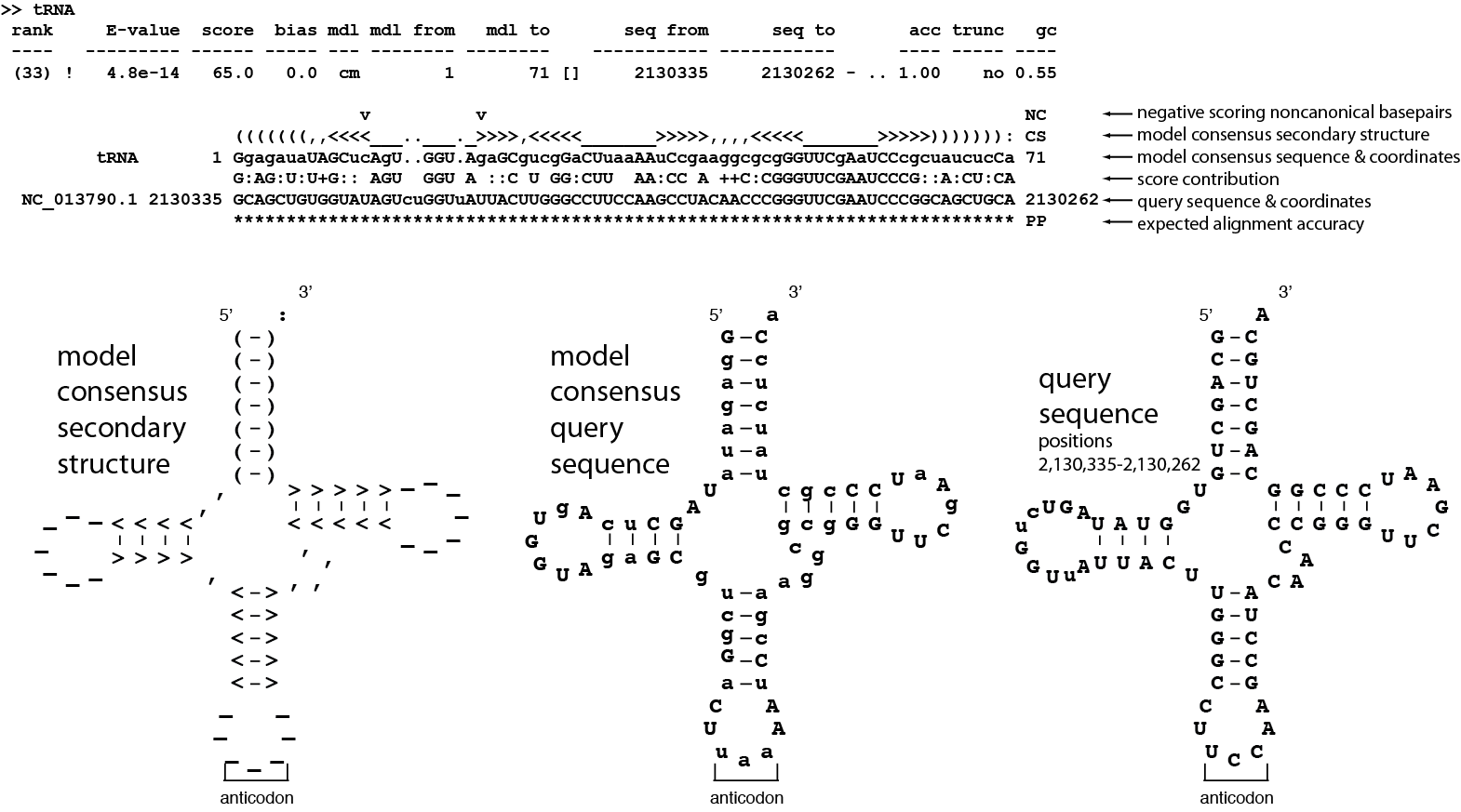
Top: cmscan standard output of alignment of hit #33. Bottom: Three secondary structure diagrams showing the relationship between the alignment and the secondary structure of the Rfam tRNA model.
The alignment contains six lines. Start by looking at the second line which ends with CS. The line shows the predicted secondary structure of the query sequence in WUSS format.
For more information see section 9 of the Infernal User’s Guide.
The secondary structure on the left above shows how the CS line folds into the tRNA cloverleaf secondary structure.
The line above the CS line ends with NC and marks negative scoring
non-canonical basepairs in the alignment with a v character. All
other positions of the alignment will be blank. More specifically, the
following ten types of basepairs which are assigned a negative score
by the model at their alignment positions will be marked with a v:
A:A, A:C, A:G, C:A, C:C, C:U, G:A, G:G, U:U, and U:C. The NC
annotation makes it easy to quickly identify suspicious basepairs in a
hit. For this example, there is a single basepair that is negative
scoring and non-canonical, it is the U:U pair between model positions
13 and 21.
The third line shows that consensus of the tRNA model. The highest
scoring residue sequence is shown. Upper case residues are highly
conserved. Lower case residues are weakly conserved or
unconserved. Dots (.) in this line indicate insertions in the target
sequence with respect to the model.
The fourth line shows where the alignment score is coming from. For a
consensus basepair, if the observed pair is the highest-scoring
possible pair according to the consensus, both residues are shown in
upper case; if a pair has a score of ≥ 0, both residues are annotated
by : characters (indicating an acceptable compensatory basepair);
else, there is a space, indicating that a negative contribution of
this pair to the alignment score. Note that the NC line will only mark
a subset of these negative scoring pairs with a v, as discussed
above. For a single-stranded consensus residue, if the observed
residue is the highest scoring possibility, the residue is shown in
upper case; if the observed residue has a score of ≥ 0, a +
character is shown; else there is a space, indicating a negative
contribution to the alignment score.
The fifth line, beginning with NC 013790.1 is the target
sequence. Dashes (-) in this line indicate deletions in the target
sequence with respect to the model.
The bottom line ends with PP. This line represents the posterior probability (essentially the expected accuracy) of each aligned residue. A 0 means 0-5%, 1 means 5-15%, and so on; 9 means 85-95%, and a * means 95-100% posterior probability. You can use these posterior probabilities to decide which parts of the alignment are well-determined or not. You’ll often observe, for example, that expected alignment accuracy degrades around locations of insertion and deletion, which you’d intuitively expect.
Alignments for some searches may be formatted slightly differently than this example. Longer alignments to longer models will be broken up into blocks of six lines each - this alignment was short enough to be entirely contained within a single block.
cmscan tabular output
The cmscan tabular output file mrum-genome.tblout contains much of
the information in the standard output, as well as some additional
information in a tabular format that is easy to manipulate using
common unix programs like grep and awk.
The top of the file has headers for each column. The first 25 hits are shown below:
 1#idx target name            accession query name           accession clan name mdl mdl from   mdl to seq from   seq to strand trunc pass   gc  bias  score   E-value inc olp anyidx afrct1 afrct2 winidx wfrct1 wfrct2 description of target
 2#--- ---------------------- --------- -------------------- --------- --------- --- -------- -------- -------- -------- ------ ----- ---- ---- ----- ------ --------- --- --- ------ ------ ------ ------ ------ ------ ---------------------
 31    LSU_rRNA_archaea       RF02540   NC_013790.1          -         CL00112    cm        1     2990   762872   765862      +    no    1 0.49  45.1 2763.5         0  !   ^       -      -      -      -      -      - -
 42    LSU_rRNA_archaea       RF02540   NC_013790.1          -         CL00112    cm        1     2990  2041329  2038338      -    no    1 0.48  46.1 2755.0         0  !   ^       -      -      -      -      -      - -
 53    LSU_rRNA_bacteria      RF02541   NC_013790.1          -         CL00112    cm        1     2925   762874   765862      +    no    1 0.49  45.1 1872.9         0  !   =       1  1.000  0.999      "      "      " -
 64    LSU_rRNA_bacteria      RF02541   NC_013790.1          -         CL00112    cm        1     2925  2041327  2038338      -    no    1 0.48  46.2 1865.5         0  !   =       2  1.000  0.999      "      "      " -
 75    LSU_rRNA_eukarya       RF02543   NC_013790.1          -         CL00112    cm        1     3401   763018   765851      +    no    1 0.49  41.5 1581.3         0  !   =       1  1.000  0.948      "      "      " -
 86    LSU_rRNA_eukarya       RF02543   NC_013790.1          -         CL00112    cm        1     3401  2041183  2038349      -    no    1 0.49  42.3 1572.1         0  !   =       2  1.000  0.948      "      "      " -
 97    SSU_rRNA_archaea       RF01959   NC_013790.1          -         CL00111    cm        1     1477  2043361  2041888      -    no    1 0.53   4.1 1552.0         0  !   ^       -      -      -      -      -      - -
108    SSU_rRNA_archaea       RF01959   NC_013790.1          -         CL00111    cm        1     1477   760878   762351      +    no    1 0.54   4.1 1546.5         0  !   ^       -      -      -      -      -      - -
119    SSU_rRNA_bacteria      RF00177   NC_013790.1          -         CL00111    cm        1     1533  2043366  2041886      -    no    1 0.53   3.7 1161.9         0  !   =       7  0.995  1.000      "      "      " -
1210   SSU_rRNA_bacteria      RF00177   NC_013790.1          -         CL00111    cm        1     1533   760873   762353      +    no    1 0.53   3.7 1156.4         0  !   =       8  0.995  1.000      "      "      " -
1311   SSU_rRNA_eukarya       RF01960   NC_013790.1          -         CL00111    cm        1     1851  2043361  2041891      -    no    1 0.53   4.6  970.4  9.9e-293  !   =       7  1.000  0.998      "      "      " -
1412   SSU_rRNA_eukarya       RF01960   NC_013790.1          -         CL00111    cm        1     1851   760878   762348      +    no    1 0.54   4.5  963.8  9.9e-291  !   =       8  1.000  0.998      "      "      " -
1513   SSU_rRNA_microsporidia RF02542   NC_013790.1          -         CL00111    cm        1     1312  2043361  2041891      -    no    1 0.53   4.6  919.9  7.7e-281  !   =       7  1.000  0.998      "      "      " -
1614   SSU_rRNA_microsporidia RF02542   NC_013790.1          -         CL00111    cm        1     1312   760878   762348      +    no    1 0.54   4.5  917.2  5.4e-280  !   =       8  1.000  0.998      "      "      " -
1715   RNaseP_arch            RF00373   NC_013790.1          -         CL00002    cm        1      303  2614544  2614262      -    no    1 0.43   0.0  184.9   1.1e-53  !   *       -      -      -      -      -      - -
1816   Archaea_SRP            RF01857   NC_013790.1          -         CL00003    cm        1      318  1064321  1064634      +    no    1 0.44   0.1  197.6   6.9e-49  !   *       -      -      -      -      -      - -
1917   FMN                    RF00050   NC_013790.1          -         -          cm        1      140   193975   193837      -    no    1 0.42   0.0  115.2   6.8e-28  !   *       -      -      -      -      -      - -
2018   tRNA                   RF00005   NC_013790.1          -         CL00001    cm        1       71   735136   735208      +    no    1 0.59   0.0   72.1   4.9e-16  !   *       -      -      -      -      -      - -
2119   tRNA                   RF00005   NC_013790.1          -         CL00001    cm        1       71  2350593  2350520      -    no    1 0.66   0.0   71.0     1e-15  !   *       -      -      -      -      -      - -
2220   tRNA                   RF00005   NC_013790.1          -         CL00001    cm        1       71  2680310  2680384      +    no    1 0.52   0.0   70.9   1.1e-15  !   *       -      -      -      -      -      - -
2321   tRNA                   RF00005   NC_013790.1          -         CL00001    cm        1       71  2351254  2351181      -    no    1 0.62   0.0   69.7   2.2e-15  !   *       -      -      -      -      -      - -
2422   tRNA                   RF00005   NC_013790.1          -         CL00001    cm        1       71   361676   361604      -    no    1 0.51   0.0   69.5   2.5e-15  !   *       -      -      -      -      -      - -
2523   tRNA                   RF00005   NC_013790.1          -         CL00001    cm        1       71  2585265  2585193      -    no    1 0.60   0.0   69.2   3.2e-15  !   *       -      -      -      -      -      - -
2624   tRNA                   RF00005   NC_013790.1          -         CL00001    cm        1       71  2585187  2585114      -    no    1 0.59   0.0   68.8   3.9e-15  !   *       -      -      -      -      -      - -
2725   tRNA                   RF00005   NC_013790.1          -         CL00001    cm        1       71  2680159  2680233      +    no    1 0.67   0.0   68.7   4.3e-15  !   *       -      -      -      -      -      - -
Each line has a whopping 27 fields. The most important ones are “seq from”, “seq to”, “strand”, “E-value”, “score”, and “target name” and “accession” (Rfam model name and accession) and “query name” and “accession” (sequence name and accession), all of which (except the two accessions) were also included in the standard output file discussed above. The meanings of these columns should be clear from their names, but for a complete explanation of these and all other fields see Section 6 (target hits table format 2) of the Infernal User’s Guide.
One column that requires explanation here is the “olp” (overlap) column, which indicates which hits overlap with one or more other hits. There are three possible characters in this column:
*This hit’s coordinates in the query sequence do not overlap with the query sequence coordinates of any other hits, on the same strand.
^Indicates that this hit does overlap with at least one other hit on the same strand, but none of those hits are “better” hits. Here, hit A is “better” than hit B, if hit A’s E-value is lower than hit B’s E-value or if hit A and hit B have equal E-values but hit A has a higher bit score than hit B.
=Indicates that this hit does overlap with at least one other hit on the same strand that is a “better” hit, given the definition of “better” above.
Removing lower-scoring overlaps from a tblout file
Using the values in the “olp” column of the tabular output file, you
can easily remove all hits that have a higher scoring overlapping
hit. This is recommended if you are annotating a genome or other
sequence dataset. To do this for the example genome annotation file
mrum-genome.tblout, and to save the remaining hits to a new file.
mrum-genome.deoverlapped.tblout, use the following grep command:
grep -v " = " mrum-genome.tblout > mrum-genome.deoverlapped.tblout
Expected running times
CM searches are computationally expensive and searching large multi-Gb genomes with the roughly 2500 models in Rfam takes hundreds of CPU hours. However, you can parallelize by splitting up the input genome sequence file into multiple files (if the genome has multiple chromosomes) and running cmscan separately on each individual file. Also, you can run cmscan with multiple threads, as explained more below.
The following timings are from Table 2 of (Nawrocki et al., 2015). All searches were run as single execution threads on 3.0 GHz Intel Xeon processors.
Genome |
Size (Mb) |
CPU time (hours) |
Mb/hour |
|---|---|---|---|
Homo sapiens |
3099.7 |
650 |
4.8 |
Sus scrofa (pig) |
2808.5 |
460 |
6.1 |
Caenorhabditis elegans |
100.3 |
20 |
5.2 |
Escherichia coli |
4.6 |
0.46 |
10.2 |
Methanocaldococcus jannaschii |
1.7 |
0.31 |
5.6 |
cmscan will run in multithreaded mode by default, if multiple processors are available. Running with 8 threads with 8 cores should reduce the running times listed in the table above by about 4-fold (reflecting about 50% efficiency versus single threaded).
Specificity
The Rfam/Infernal approach aims to be sufficiently generic to cope with all types of RNAs. A sequence can be searched using every model in exactly the same way.
In contrast, several tools are available that search for specific types of RNA, such as
tRNAscan-SE for tRNAs
RNAMMER for rRNA
snoscan for snoRNAs
SRPscan for SRP RNA
The generic Rfam approach has obvious advantages. However, the specialised programs often incorporate heuristics and family-specific information which may allow them to out-perform the general method. A comparison of Infernal versus some of these generic methods is presented in section 2.2 of a 2014 paper (by one of the authors of Infernal), available here.
Pseudogenes
ncRNA derived pseudogenes pose the biggest problem for eukaryotic genome annotation using Rfam/Infernal. Many genomes contain repeat elements that are derived from a non-coding RNA gene, sometimes in huge copy number. For example, Alu repeats in human are evolutionarily related to SRP RNA, and the active B2 SINE in mouse is recently derived from a tRNA.
In addition, specific RNA genes appear to have undergone massive pseudogene expansions in certain genomes. For example, searching the human genome using the Rfam U6 family yields over 1000 hits, all with very high score. These are not “false positives” in the sequence analysis sense, because they are closely related by sequence to the real U6 genes, but they completely overwhelm the small number (only 10s) of expected real U6 genes.
At present we don’t have computational methods to distinguish the real genes from the pseudogenes (of course the standard protein coding gene tricks - in frame stop codons and the like - are useless). The sensible and precedented method for ncRNA annotation in large vertebrate genomes is to annotate the easy-to-identify RNAs, such as tRNAs and rRNAs, and then trust only hits with very high sequence identity (>95% over >95% of the sequence length) to an experimentally verified real gene. tRNAscan-SE has a very nice method for detecting tRNA pseudogenes.
Danger
We recommend that you use Rfam/Infernal for vertebrate genome annotation with extreme caution!
Nevertheless, Rfam/Infernal does tell us about important sequence similarities that are effectively undetectable by other means. However, in complex eukaryotic genomes, it is important to treat hits as sequence similarity information (much as you might treat BLAST hits), rather than as evidence of bona fide ncRNA genes.